## [A ȷupyter notebook](http://pdes-net.org/scripts/indices.tar.xz)
Scientists move in mysterious ways, particularly when they try to measure their individual performance as a scientist. As I've explained in a [previous post](http://pdes-net.org/cobra/posts/rsums-and-indices.html), the most popular and commonly accepted of these measures is the [h index](http://en.wikipedia.org/wiki/H-index) $\mathcal{H}$, which has been declared to be superfluous on both [empirical](http://michaelnielsen.org/blog/why-the-h-index-is-virtually-no-use/) and [mathematical](http://www.ams.org/journals/notices/201409/rnoti-p1040.pdf) grounds. Either of these references relates $\mathcal{H}$ to the square root of the total number of citations $\mathcal{N}$, the first one approximately
$\mathcal{H} \approx 0.5 \sqrt{\mathcal{N}}$
and the second one exactly:
$\mathcal{H}=\sqrt{6}\log{2}\sqrt{\mathcal{N}}/\pi \approx 0.54 \sqrt{\mathcal{N}} $.
Since I anyway wanted to test [pandas](http://pandas.pydata.org/), [seaborn](https://stanford.edu/~mwaskom/software/seaborn/) and [statsmodel](http://statsmodels.sourceforge.net/), I gathered $\mathcal{H}$, $\mathcal{N}$, and the i10 index $\mathcal{I}$ from all my coauthors on Google Scholar. It turned out that not even a quarter of my coauthors have a Google Scholar account, but I figured that 71 data points would provide an acceptable statistics.
```python
%matplotlib inline
import pandas as pd
import numpy as np
import matplotlib as mpl
import matplotlib.pyplot as plt
import statsmodels.formula.api as sm
import seaborn as sns
```
```python
# read data into a Pandas DataFrame
data = pd.read_table("/home/cobra/ownCloud/MyStuff/projects/python/publishing/hindex.dat")
# check the data head
data.head()
```
|
Citations |
Hindex |
i10index |
| 0 |
952 |
12 |
17 |
| 1 |
1913 |
20 |
35 |
| 2 |
5327 |
34 |
151 |
| 3 |
650 |
13 |
14 |
| 4 |
3855 |
25 |
68 |
Looks all right.
```python
logdata = np.log10(data)
```
The correlation of the data is much more clear when displayed logarithmically:
```python
vars = ["Citations", "Hindex", "i10index"]
sns.pairplot(logdata, vars=vars, size=3, kind="reg");
```
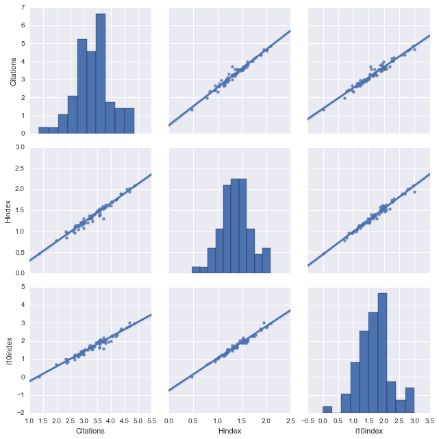
Now look at *that!* Two lines of code and seaborn visualizes all correlations in my data set. The diagonal elements of this 3x3 matrix plot show the distributions of $\mathcal{N}$, $\mathcal{H}$, and $\mathcal{I}$ (which seem to be close to normal distributions), and the off-diagonal elements visualize their correlations emphasized by a linear regression (kind="reg"). And how correlated they are! There's indeed no need for a definition of 'indices' if the number of citations is all what it boils down to.
Seaborn is great for visualization, as we have seen, but for quantitative statistical information, it's better to use statsmodel:
```python
hc = sm.ols(formula='Hindex ~ Citations', data=logdata)
fithc = hc.fit()
ic = sm.ols(formula='i10index ~ Citations', data=logdata)
fitic = ic.fit()
hi = sm.ols(formula='Hindex ~ i10index', data=logdata)
fithi = hi.fit()
```
Let's compare the slope of our data with that predicted above:
```python
fithc.params.Citations
```
0.45708354021378172
```python
np.sqrt(6)*np.log(2)/np.pi
```
0.54044463946673071
Solid state phycisists have to work harder!
One can get also get more information, if desired:
```python
fithi.summary()
```
OLS Regression Results
| Dep. Variable: | Hindex | R-squared: | 0.974 |
| Model: | OLS | Adj. R-squared: | 0.974 |
| Method: | Least Squares | F-statistic: | 2592. |
| Date: | Mon, 16 May 2016 | Prob (F-statistic): | 1.84e-56 |
| Time: | 14:42:47 | Log-Likelihood: | 114.08 |
| No. Observations: | 71 | AIC: | -224.2 |
| Df Residuals: | 69 | BIC: | -219.6 |
| Df Model: | 1 | | |
| Covariance Type: | nonrobust | | |
| coef | std err | t | P>|t| | [95.0% Conf. Int.] |
| Intercept | 0.4498 | 0.019 | 23.723 | 0.000 | 0.412 0.488 |
| i10index | 0.5454 | 0.011 | 50.910 | 0.000 | 0.524 0.567 |
| Omnibus: | 3.438 | Durbin-Watson: | 2.391 |
| Prob(Omnibus): | 0.179 | Jarque-Bera (JB): | 2.600 |
| Skew: | -0.408 | Prob(JB): | 0.273 |
| Kurtosis: | 3.462 | Cond. No. | 7.44 |
And of course, we can display these fits independent of seaborn:
```python
xlist_cit = pd.DataFrame({'Citations': [logdata.Citations.min(), logdata.Citations.max()]})
xlist_i10 = pd.DataFrame({'i10index': [logdata.i10index.min(), logdata.i10index.max()]})
```
```python
preds_hcit = fithc.predict(xlist_cit)
preds_hcit;
preds_i10cit = fitic.predict(xlist_cit)
preds_i10cit;
preds_hi10 = fithi.predict(xlist_i10)
preds_hi10;
```
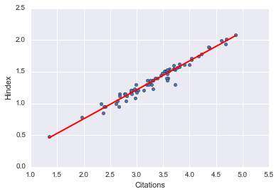
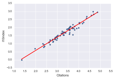
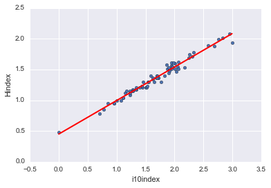
```python
logdata.plot(kind='scatter', x='Citations', y='Hindex')
plt.plot(xlist_cit, preds_hcit, c='red', linewidth=2);
logdata.plot(kind='scatter', x='Citations', y='i10index')
plt.plot(xlist_cit, preds_i10cit, c='red', linewidth=2);
logdata.plot(kind='scatter', x='i10index', y='Hindex')
plt.plot(xlist_i10, preds_hi10, c='red', linewidth=2);
```